SketchRNN with Attention
Tweaking SketchRNN (LSTM-VAE) with attention! And generating owl drawings.
TLDR
In this project we explore Sequence-to-Sequence VAE to generate simple sketch drawings as a sequence of strokes. We improve upon existing work by using attention mechanism in the decoder. We show that proposed improvement gives benefits in training time while does not degrade the quality of generation. We discover that training time is an issue, as RNN are hardly parallelizible and SketchRNN is expensive to train. Improving convergence speed allows for more efficient training sessions, achieving the same validation scores with 40% time reduction.
We also tried training on a more complex, yet shallow dataset of sketches from DoodlerGAN, but the results are inconclusive. More work is required here.
Code: github repository
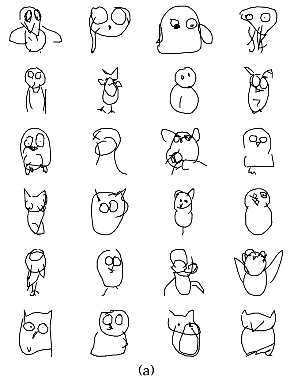
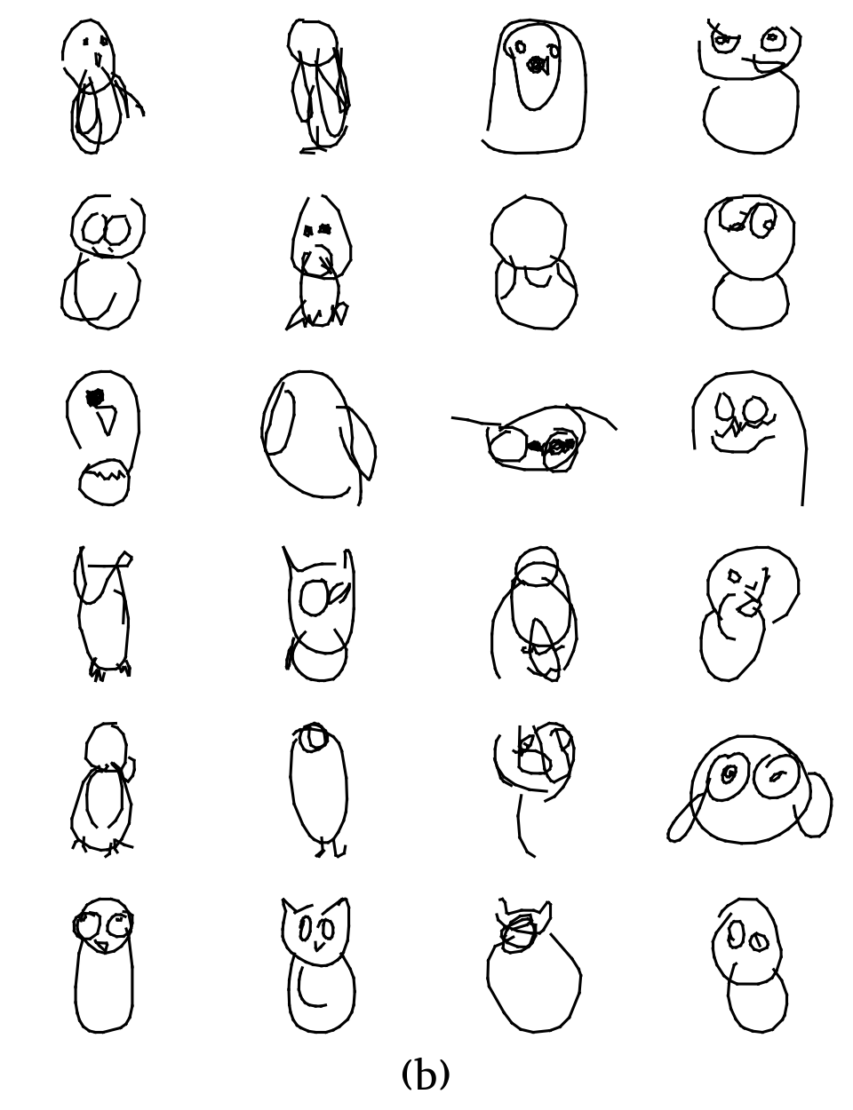
Disclaimer: this little project was done as a course project for IFT6010: Modern NLP. It is far from complete, I wish I had another month to tinker around. Anyway, I decided to put online for anyone interested.
If you already know about SketchRNN, go right to Experiments.
Motivation
Sketches are a natural part of our world from our daily life to professional practice. They play an essential role in any design process: rough pen-and-paper sketches are easy to produce, yet they are expressive enough to convey the idea. Contrary to realistic images, sketches are inexact and abstract.
Sketch-RNN paper
Note that in SketchRNN the final drawing is constructed as a set of polygonal chains. To get an image we rasterize lines on a canvas. This is a particular case of a more general vector graphics format, when image is stored as a set of primitives with drawing parameters (color, line width, etc.).
Many sketch generation works focused on raster image generation, representing images as array of pixels. See this github collection of Sketch Synthesis papers for a general overview. In the recent work
Proposed idea
Motivated by advancements in Natural Language Processing using attention mechanism, we propose an improved SketchRNN model with attention. The goal of this project is to train an improved model and compare it with the baseline.
Baseline: Sketch-RNN
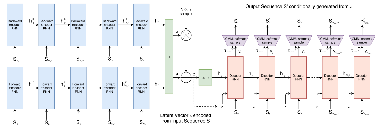
SketchRNN
Encoder is an unsupervised bidirectional RNN
Having latent code $z \in \mathbb R^{128}$ we then perform decoding. Decoder is a uni-directional auto-regressive RNN, that takes as input previous state and latent code. The outputs are passed as a parameters to $M=20$ Gaussian mixture models ($\Pi, \mu_x, \mu_y, \sigma_x, \sigma_y, \rho_{xy}$ for each of $M$ GMMs, $\sum \Pi = 1$) and we extract new offset vector $(\Delta x, \Delta y)$ as a sample from GMMs distribution. Pen state vector is extracted as a softmaxed projection of the decoder output. During training, we know the ground truth sequence, and next step of decoder is provided with correct input. During evaluation, the output point embedding of the previous step is passed to the input of the next step.
Loss is a weighted sum of two terms: one is reconstruction loss $L_{R}$ (how well we reconstructed the starting sample) and Kullback-Leibler divergence loss $L_{KL}$ (how close the distribution of $z$ is to $\mathcal N(0,1)$).
\[L = L_R + w_{KL} \cdot L_{KL}\]In our experiments, $w_{KL}=0.5$. During training, we use annealing term to mitigate KL loss influence in the beginning of the training.
\[\eta_{step} = 1 - (1-\eta_{min}) R^{step}\] \[L_{training} = L_R + w_{KL} \cdot \eta_{step} \cdot \max (L_{KL}, 0.2)\]Reconstruction loss has two terms: loss for the offset $L_s$ and pen state $L_p$
\[L_s = - \frac 1 {N_{max}} \sum_{i=1}^{N_s} \log (\sum_{j=1}^M \Pi_{j,i} \cdot \mathcal N(\Delta x, \Delta y | \mu_{x,j,i}, \mu_{y,j,i}, \sigma_{x,j,i}, \sigma_{y,j,i}, \rho_{xy,j,i}))\] \[L_{p} = - \frac 1 {N_{max}} \sum_{i=1}^{N_{max}} \sum_{k=1}^3 p_{k,i} \log (q_{k,i})\]And Kullback-Leibner divergence can be interpreted as the parameter difference with the normal distribution. Original paper proposes this loss term:
\[L_{KL} = - \frac{1}{2N_z} (1 + \hat \sigma - \mu^2 - \exp (\hat \sigma) )\]Experiments
The backbone of our model remains the same as in SketchRNN, although original paper used more complex HyperLSTM, while we use LSTM to save computations (otherwise it would be infeasible given the time constraints and resources available). We use the same reconstruction loss and Kullback-Leibner divergence. However, due to numerical limitations we use smaller model (with 256 hidden states in encoder and 512 in decoder).
Attention in decoder
We utilize dot-product attention from
Now at each time step the decoder network receives latent code $z$, previous point embedding, and a context vector $\in \mathbb R^{64}$, that is computed on all the previous points embeddings.
Note that as we are in auto-regressive model setup, our attention context must not see the future token. During training we achieve this by masking alignment scores with $-\infty$ (this is required such that the softmax contribution of masked tokens is exactly 0). During evaluation, attention context vector is computed on the go. This attention mechanism is somewhat similar to XL-Net autoregressive attention (they do a two-stream attention for permuted language modeling).
Context vector is computed by using query, key and value projections of starting embeddings $\in \mathbb R^5$, and combining them into scaled dot-product attention:
\[\text{Attention} (Q,K,V) = \text{softmax} (\frac{QK^\top}{\sqrt{n}}) V\]We experimented with positional encoding, but found that it adds no effect neither to quality nor to the speed of convergence. We argue that in these low-dimensional input representations positional encodings do not convey any useful information.
Although attention requires additional computations, during training it is highly parallelizible, as we already new all the inputs to decoder RNN, and proper masking ensure that future data does not leak into current step. In our setting, computing attention added 5 seconds to the epoch computation time (37 compared to 32 seconds, 15% increase).
Dataset
- “Quick, draw!” dataset used in
, category owl: 75,000 sketches, train / validation / test : 70,000 / 2500 / 2500 google cloud link - “Creative Birds” from
: 10,000 sketches. Splitted as 8500 / 1000 / 500. Transformed from the original dataset, can be found in our repository
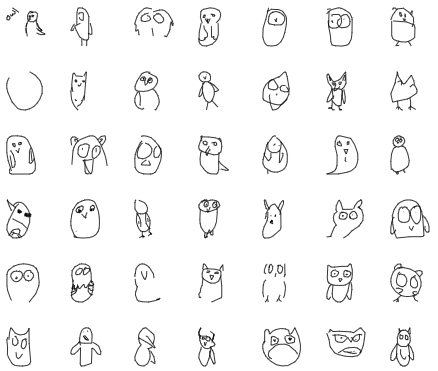
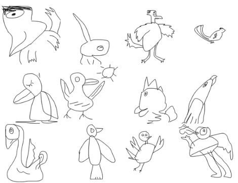
Preprocessing: fixed-size normalization (each sketch is contained in 256x256 window), deleting short strokes, line simplification (Ramer–Douglas–Peucker algorithm). Each stroke point will be encoded as $(\Delta x, \Delta y, p_1, p_2, p_3)$, where $p_i$ is a pen status after the corresponding point (pen up, pen down, end of sketch), and the length is padded to 200 by repeating the token (0,0,0,0,1). Sequences longer than 200 are discarded. For QuickDraw, simplification was already done, corresponding operations were performed for CreativeBirds data.
Training setup
We compare the basaeline model with our improved SketchRNN-Attention model. Models were trained under the same hyperparameters, with learning rate 0.0001, batch size 100, with fixed random seed. We compare the models by loss values on validation set, as there is no better numerical metric to evaluate sketch quality.
The models were trained for 1000 epochs (or until gradient explosion occurs, making loss NaN). For Creative Birds, as it is 7 times smaller, maximum number of epochs was set to 3000. Then the best model was chosen according to the validation loss.
Each experiment took about 10 hours of training on NVidia RTX 2080 Ti.
Results
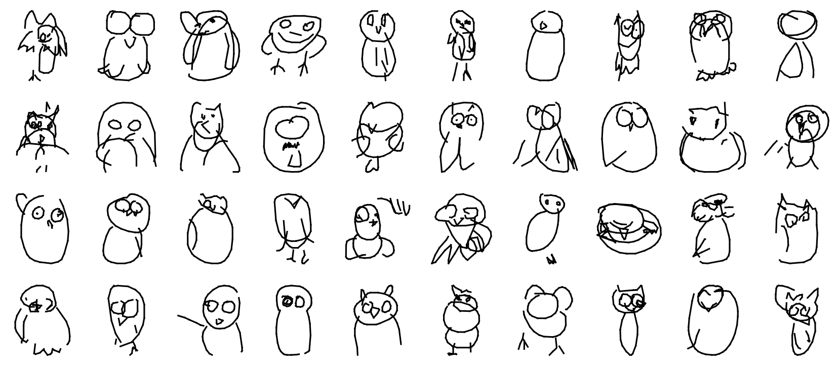
Training SketchRNN turned out to be a challenging problem. After we cleaned all bugs in our code (the loss is particularly tricky to implement, and we took an open-source implementation after days of suffering), the training time comes to play. As we compute time-steps in RNN sequentially, they are slower to compute than typical convnets. Because of recurrence, “gradient explosion” problem exists, which result in NaN exceptions and training termination. We tryied dozens of training setups with different datasets (sketches classes, like bird, cat, and also dataset size) and hyperparameters (learning rate, hidden size, annealing )
Interpolation
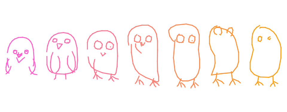
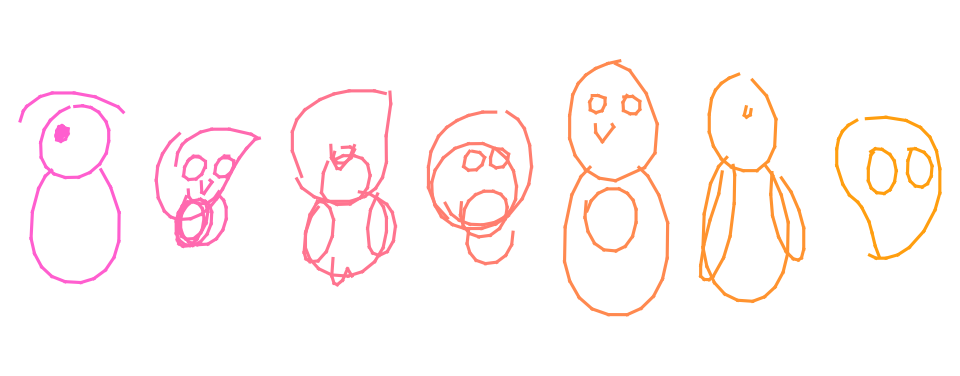
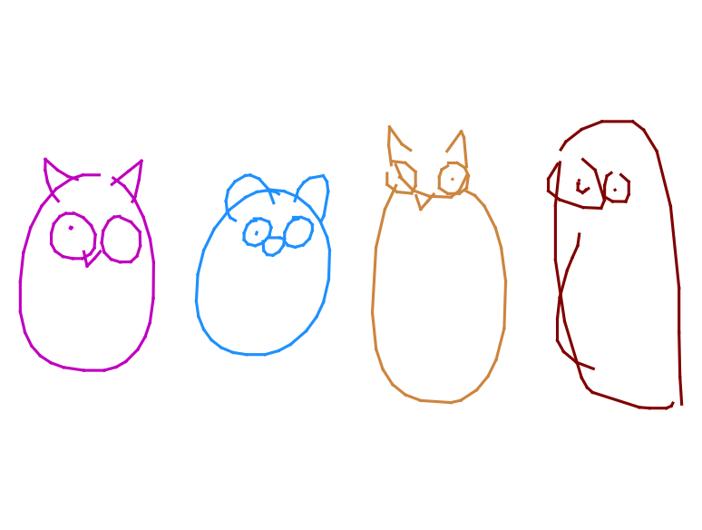
We can interpolate between sketches using trained model and latent codes.
Latent space arithmetic
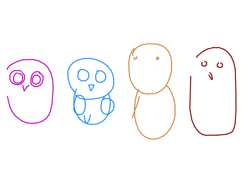
Original paper reports some nice properties of a large models trained on multiclass generation (see inset). We did not find good examples of latent space arithmetic in either of our models. One explanation may be that our models are too simple (see underfitting). Alternatively, arithmetic may be a property of a multi-class generative models.

Training on CreativeBirds
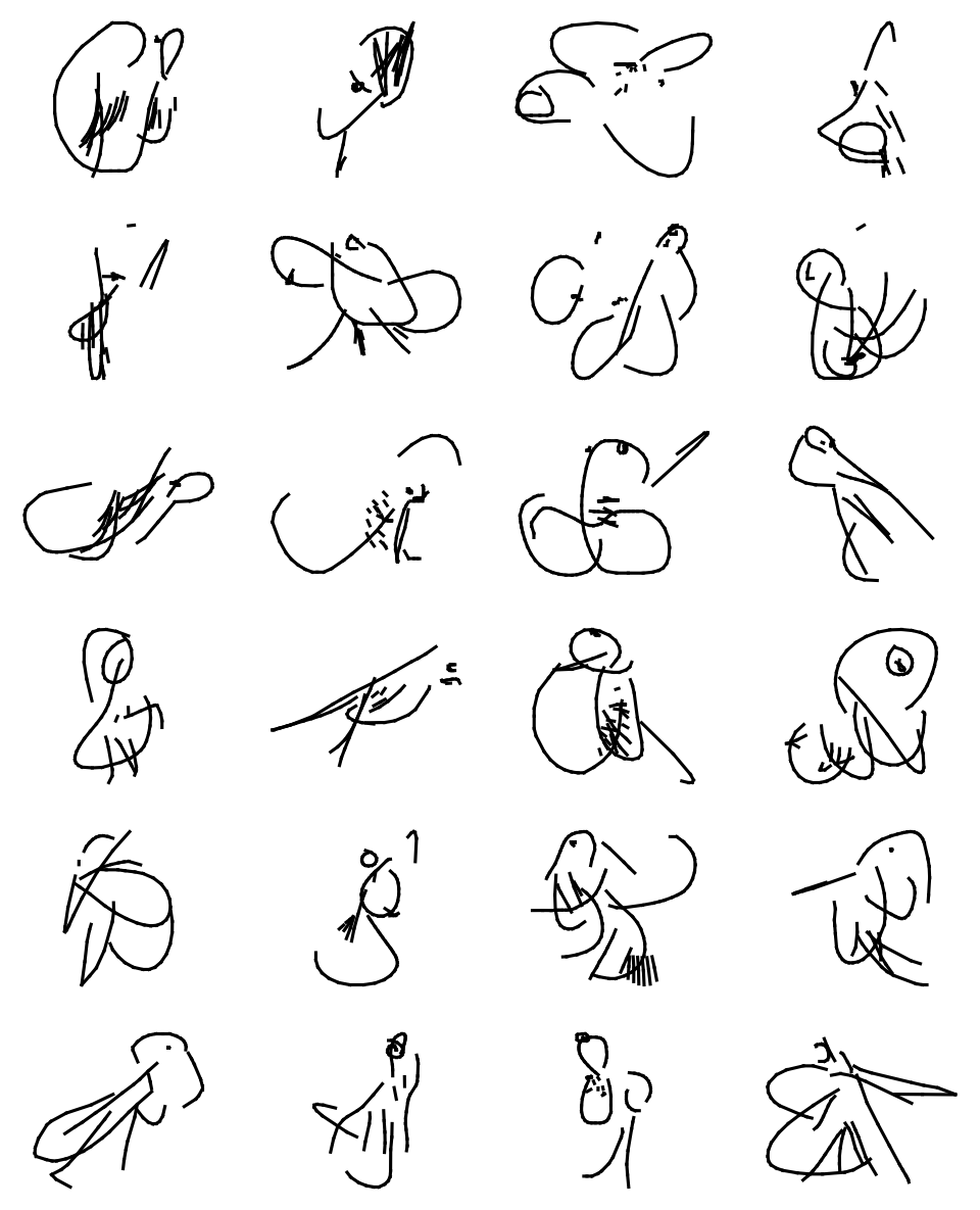
Althiugh showing good numbers in loss, training on Creative Birds dataset was not successfull: generated samples are far from the fround truth one. The authors of the original paper also noted that model suffers when training on complex data classes (like lobster or mermaid):
“The models trained on these more challenging image classes tend to draw smoother, more circular line segments that do not resemble individual sketches, but rather resemble an averaging of many sketches in the training set.”
I our case, the data is both complex and sparse, as Creative Birds contains only 8500 sketches opposed to 70,000 in Quickdraw. Despite showing good loss values (table below), our trained model does not produce bad sketches (see inset). This is a challenging problem for future research: we can try increasing the model size, mixing the datasets together, additional data preprocessing for Creative Birds dataset, etc.
Speedup
To show convergence benefits of using attention we compare 2 pair of experiments on each of our datasets.
Experiments table on QuickDraw owl data:
| Model | $h_{enc}$ | $h_{dec}$ | best epoch | $L_R$ | $L_{KL}$ |
|---|---|---|---|---|---|
| Baseline | 256 | 512 | 761 | -0.25 | 0.21 |
| Attention | 256 | 512 | 420 | -0.24 | 0.24 |
Experiments table on Creative Birds data:
| Model | $h_{enc}$ | $h_{dec}$ | best epoch | $L_R$ | $L_{KL}$ |
|---|---|---|---|---|---|
| Baseline | 256 | 512 | 1977 | -0.8 | 0.31 |
| Attention | 256 | 512 | 1002 | -1.44 | 0.64 |
Validation loss curves on owl: baseline (blue) and attention (orange) models.

Underfitting
Note that quantitative and qualitative results of baseline and attention models are very similar. However, the final scores are far from what is reported in the original paper (see inset).
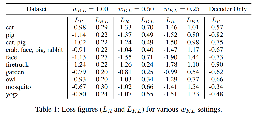
We conclude that our models are too simple for the data. Unfortunately, increasing model size comes at a huge computational cost. We tried training larger model (512 units in encoder, 1024 units in decoder) for 28 hours (1000 epochs) on QuickDraw cat data, which resulted in overfitting on training data.
Conclusions
In this work we improved existing sequence-to-sequence VAE model on sketch generation by adding auto-regressive attention. It drastically improved training time, and also showed slight visual improvements. We conducted a small ablation study to confirm the results. As it turned out, replicating the results from the existing paper \cite{sketchrnn} takes massive computational resources, so the proposed improvement is quite useful.
Although model failed to generalize on the new complex dataset, it did not fail into “mode collapse” state. The results are still diverse and detailed, which suggests that more training is requires. The same can be said for a simpler “owl” class model – generated results are still not perfect, but with more computations we see no obstacles to replicate and even surpass the results from the original paper.
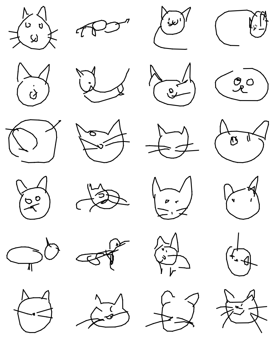
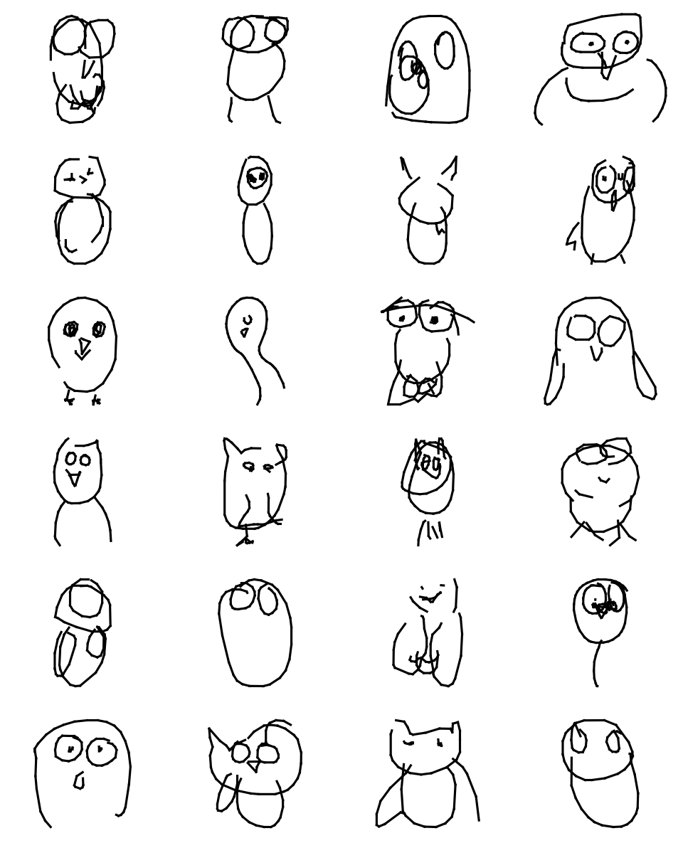
Gallery
More Posts
Here are some more articles you might like to read next: